

Cover Image: Solitary wave in a laboratory wave channel – author: Christophe.Finot et Kamal HAMMANI / licensed under CC BY-SA 2.5
Table of Contents
People have known about waves pretty much forever. We probably noticed them first on the surface of water, which makes sense — it’s right there in front of you. The soliton wave, though, is a different story. Nobody spotted one until the 19th century. And since then, this strange type of wave motion has turned up in places no one expected: out in the vast reaches of the universe, down at the molecular level, and even deeper than that — in the structure of space itself and in elementary particles.
What Is a Soliton Wave?
So what’s a wave, exactly? It’s a type of motion in a material medium where the particles oscillate around their equilibrium positions while staying connected to their neighbors by elastic forces. Because those forces exist, the oscillation of the first excited particle gets passed along to the particles next to it, and an elastic wave forms. A few things are worth knowing here. If you combine several waves with different frequencies and/or amplitudes, you get a new wave — and it can look completely different from the waves that went into making it. This kind of stacking can produce a wave formation shaped like a big hill (usually trailed by a series of much smaller crests), what’s called a “wave impulse.” Energy travels along with the moving pulse. Now, this might remind you of a tsunami, but a wave impulse built by stacking up linear waves can’t actually describe that kind of moving water mass. The reason is dispersion. Linear waves disperse, so the impulses they form fall apart pretty quickly — or, as a physicist would put it, their “lifetime” is too short to cover any real distance and deliver destructive energy.

Image credit: Kraaiennest / CC BY-SA 4.0 (via Wikimedia Commons)
The Translatory Wave: John Scott Russell’s Discovery
In August 1834, a Scottish engineer named John Scott Russell was watching a barge being pulled by horses along a narrow canal. At some point the barge stopped — but the mass of water that had been pushed along in front of it kept going. A larger heap of water built up in front of the bow, then suddenly shot forward at high speed, leaving the barge far behind. This round, smooth, clearly defined mound of water just kept rolling down the canal without visibly changing shape or slowing down. Russell chased the strange wave on horseback, and it only lost its shape after a few kilometers. He was so struck by what he’d seen that he started studying it right away, and he gave it a name: the translatory wave.
Russell’s Wave Tank Experiments and the Solitary Wave
The canal in question, by the way, was the Union Canal near Edinburgh — and it has a small place in scientific history because of that day. In fact, the observation was considered important enough that in July 1995, a group of scientists gathered at an aqueduct on that same canal (now named the Scott Russell Aqueduct, near Heriot-Watt University) and recreated the solitary wave in honor of the man who first described it.
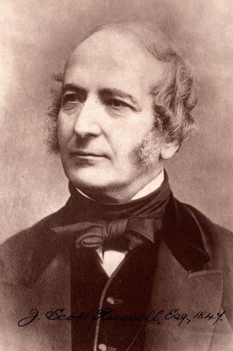
Image credit: Unknown author / public domain
By Russell’s time, the basic principles of hydrodynamics had already been worked out and put into mathematical language. Leonhard Euler (1707-1783) did this work in 1755, and Claude Louis Navier (1785-1836) followed in 1822. So Russell didn’t stop at simply describing translational waves. He ran a whole series of experiments on water, measuring wave speeds — the measurements were taken in the Firth of Forth and on the river Dee in Cheshire. He went even further than field observations, though. Russell built a wave tank in his own back garden, roughly 30 feet long, where he could generate solitary waves on demand by dropping a weight at one end of the channel. Those controlled experiments let him pin down something remarkable: an empirical formula for the wave’s speed. The speed squared turned out to be proportional to the sum of the channel depth and the wave height (c² = g(h + a), where g is the acceleration due to gravity, h is the depth of the water, and a is the amplitude of the wave). In plain terms: taller waves move faster. That one detail — speed depending on amplitude — is exactly what separates these waves from ordinary linear ones, and it would turn out to be the key to the whole story.
After pulling all his observations together, Russell laid out the following properties of translational waves:
- the speed and shape of the translational wave do not change
- the speed depends on the height of the wave crest and the depth of the channel (the height of the crest has to be less than the depth of the channel)
- a big enough wave will split into two (or more) waves, and it works like this: the wave “sheds” its excess mass and leaves it behind. The wave that splits off moves slower than the “parent” wave
- when two large translational waves meet, they pass right through each other without changing shape or speed
He also sorted the movements of the water mass into four orders and two groups of waves: solitary and gregarious. Capillary waves and surface waves went into the gregarious group, and he later started calling translatory waves “great solitary waves.” The idea of a solitary wave has stuck around to this day — it basically means any flat wave impulse (usually bell-shaped) that moves in one direction and holds its shape.
Russell published his results in 1844, in his now-famous “Report on Waves” for the British Association for the Advancement of Science. They eventually caught the attention of plenty of physicists, who tried to describe them analytically. Interestingly, Hamilton — who knew wave physics well and was on friendly terms with Russell — stayed out of the whole discussion. He was busy at the time with his own new discovery, the Quaternions.
Skeptics, Supporters, and the Korteweg-de Vries Equation
Plenty of critics showed up too, doubting whether Russell’s conclusions were right and whether translational waves even existed. The most prominent skeptics were George Biddell Airy (1801-1892), the Astronomer Royal, whose own theory of shallow-water waves said that a wave like Russell’s couldn’t keep its shape, and George Gabriel Stokes (1819-1903), whose equations every hydrodynamics student knows today. From the standpoint of the linear wave theories available at the time, the critics actually had a point — nothing in their mathematics allowed a wave to travel that far without falling apart. The problem wasn’t Russell’s observations; it was that the theory of the day simply wasn’t equipped to handle nonlinearity.

Image credit: Kraaiennest / CC BY-SA 3.0 (via Wikimedia Commons)
Russell’s reputation got its first real boost from theory in the 1870s. Joseph Boussinesq (1842-1929) derived equations describing shallow-water waves in the 1870s, with his major work published in 1877, and Lord Rayleigh (1842-1919) independently published a solution for the solitary wave in 1876 — both confirming, mathematically, that the wave Russell chased down the canal could exist after all. Still, the definitive word came later. It wasn’t until 1895 that someone derived and solved partial differential equations that could fully describe Russell’s waves. That work came from Professor Diederik Johannes Korteweg (1848-1941) of the University of Amsterdam and his student Gustav de Vries (1866-1934). Today we know these as the Korteweg-de Vries (KdV) equations. Their equation balances exactly the two effects we keep running into in this story — dispersion and nonlinearity — and its solitary-wave solution has the elegant bell shape of a squared hyperbolic secant (the sech² profile), with the amplitude, width, and speed all locked together: taller solitons are narrower and faster.
Sadly, Russell didn’t live to see his waves vindicated — he died in 1882, more than a decade before Korteweg and de Vries published. He spent much of his later career as a naval engineer, where his “wave-line” theory of hull design influenced shipbuilding, and he was involved in the construction of the Great Eastern, the largest ship of its time.
1834: A Remarkable Year for Science
It’s worth pausing on 1834 for a second, because the discoveries from that single year still shape science today. That year, the Irish mathematician William Rowan Hamilton put the equations of classical mechanics into canonical form and discovered an optical-mechanical analogy — something that later played a big role in laying the theoretical groundwork for quantum mechanics. The same year, Clapeyron presented the work of Sadi Carnot to the scientific public, which had a real impact on the development of thermodynamics. Michael Faraday discovered the laws of electrolysis that year and predicted the existence of elementary charge. The English mathematician Charles Babbage worked out the basic principles of his “analytical machine,” which influenced the later development of computers. And finally, that same year, a soliton was observed for the first time, near Edinburgh.
What Do Fermi, Pasta, Ulam, the Manhattan Project, and the Solitons Have in Common?
The famous nuclear physicist Enrico Fermi (1901-1954) stepped away from research tied to the US nuclear program in the early 1950s. He stayed in touch, though, with two of his associates at the Los Alamos laboratories, John Pasta (1918-1981) and Stanislaw Ulam (1909-1984) — mostly because Los Alamos had a newly built calculating machine designed for numerically solving certain problems. That machine was MANIAC, built primarily for the demanding calculations of the weapons program — which is where the Manhattan Project enters this story. The machine needed testing, and it needed a task that would really push its resources. So Fermi suggested tackling a problem Peter Debye had posed long before: explaining the finite thermal conductivity of solids. For their model, they took an anharmonic chain — 32 balls of a given mass connected by springs. When stretched, the springs acted on the masses with a force that had two components: a linear one following Hooke’s law (proportional to the first power of the spring’s elongation) and a much weaker force proportional to the second power of the elongation. The calculations were programmed and run on the MANIAC computer by Mary Tsingou, which is why the problem these days is increasingly called the Fermi-Pasta-Ulam-Tsingou (FPUT) problem.
The Experiment That Refused to Thermalize
Here’s the background. When you excite just one mode of oscillation in a system of particles connected by elastic springs (a mode with one precisely defined frequency), the energy you put in stays in that mode indefinitely. Other modes at other frequencies never get excited — the system just keeps oscillating the same way, forever. Fermi was convinced that if you excited the lowest mode in the system (the one with the lowest frequency and the maximum wavelength), then thanks to that small nonlinear component in the interaction, the excitation energy would slowly leak into higher modes, gradually waking them up. This redistribution of energy should keep going until the total excitation energy was spread evenly across all the harmonics. In other words, Fermi expected the system to reach thermodynamic equilibrium — or, as physicists like to say, to thermalize. That outcome would have lined up with how certain nonlinear systems (the ones known at the time) were understood to behave. The result should be a system oscillating in a complicated way that doesn’t look anything like a sine function.
At first, the computer’s calculations matched Fermi’s expectations. But one day, the machine was left running for a long stretch. When Fermi’s associates came back to the computer room, they got a surprise. After several periods of the basic mode, almost all of the excitation energy had gathered back into that mode again! The system was stubbornly refusing to thermalize. These unexpected results — written up in a Los Alamos report in 1955, after Fermi’s death — kicked off further research into nonlinear systems, and out of that work grew two modern fields of physics: soliton theory and chaos theory. Not bad for what started out as a stress test for a new computer.
From Plasma Physics to the Name “Soliton”
Universal phenomena have a habit of popping up unexpectedly, not just across different areas of physics but in other sciences too. Sure enough, solitons soon showed up in plasma physics. In the late 1950s, Roald Zinnurovich Sagdeev developed the theory of shock waves in plasma. Waves like these form, for example, when the solar wind flows around the Earth. Sagdeev noticed that waves similar to the ones Russell had watched on the water’s surface could form here as well.
Physicists Martin Kruskal (1925-2006) and Norman Zabusky (1929-2018) were also working on plasma physics. They noticed something neat: if you let the number of particles in the Fermi, Pasta, and Ulam chain grow without limit, the chain starts to resemble a (continuous) nonlinear string — and its small oscillations are described by… the KdV equation (Korteweg-de Vries)! Which means the lack of energy thermalization in the chain is tied to the stability of the soliton that forms in it. And the soliton doesn’t change shape as it travels along the chain. Kruskal and Zabusky also ran some additional numerical experiments and saw that a collision between two solitons is a genuinely complex event, with an outcome that depends on a lot of physical factors. When two localized wave impulses made of linear waves collide, they combine in the area where they meet and then carry on moving independently, as if they’d never crossed paths at all. With soliton impulses, things work differently — and in this case, the mathematical tools developed for describing linear waves (the ones based on Fourier analysis) simply stop working.
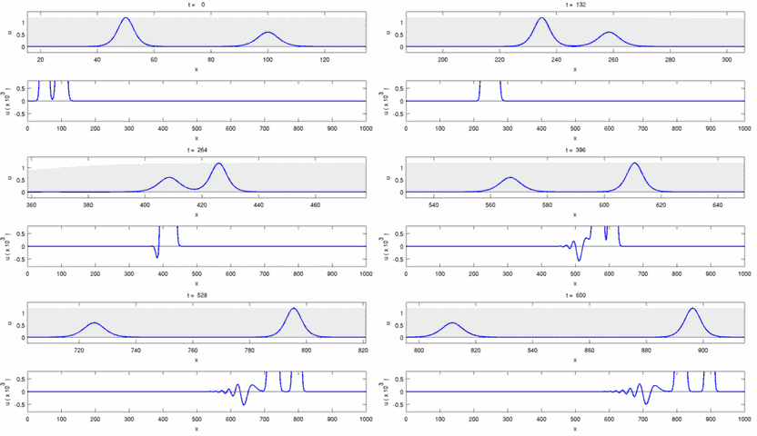
The upper graph is for a frame of reference moving with the average velocity of the solitary waves.
The lower graph (with a different vertical scale and in a stationary frame of reference) shows the oscillatory tail produced by the interaction.[11] Thus, the solitary wave solutions of the BBM equation are not solitons.
Image credit: Kraaiennest / CC BY-SA 3.0 (via Wikimedia Commons)
The theory of soliton interactions is its own branch of wave physics. For solitons that solve the KdV equation, what happens when two of them collide comes down to the ratio of their velocities. If the velocity ratio is greater than 3, the two soliton pulses first merge and then separate, keeping their original shape and speed. Sound familiar? That’s exactly the behavior Russell noticed in his experiments about a century earlier. If the velocity ratio is less than 3, the waves first “bounce” off each other and then change both their speed and their shape. In both cases, you can spot a certain jump in the position of both the faster and the slower soliton pulse — a phase shift, which is essentially the only lasting trace the collision leaves behind. The mathematician Peter Lax later put this two-soliton interaction on rigorous footing, classifying the possible types of collision in a 1968 paper that also introduced what are now called Lax pairs — a structure that became one of the central tools of soliton mathematics.
Fortunately, the research didn’t stop at numerical calculations. In 1967, Gardner, Greene, Kruskal, and Miura found a way to obtain exact solutions of nonlinear equations of the KdV type, which made it possible to explain the results Fermi, Pasta, and Ulam had gotten. Their technique, known today as the inverse scattering transform, was a genuine breakthrough — it did for certain nonlinear equations roughly what the Fourier transform does for linear ones, and it opened the floodgates for solving a whole family of nonlinear equations that had previously looked hopeless. Two years before that, in their famous 1965 paper, Zabusky and Kruskal had proposed the name “soliton” and brought it into physics. The name was deliberate — the “-on” ending echoes particle names like electron, proton, and photon, because they wanted to highlight the similarity they’d discovered between the properties of solitons and particles.
That said, the early attempts to explain statistically why energy doesn’t flow from the primary harmonic into the higher ones all failed. The first real success came when an adapted version of the Krylov and Bogolyubov averaging method was applied to the problem, in the first half of the 1960s.
How Is a Soliton Wave Formed?
The concept of dispersion was brought into the physics of linear waves by Isaac Newton. The term refers to how the propagation speed of a wave’s phase depends on its wavelength (or oscillation frequency). Dispersion is behind the scattering of wave packets, the uneven movement of wavefronts, and plenty of other phenomena. You’ve seen dispersion in action, by the way, every time you’ve looked at a rainbow or watched sunlight split apart in a prism — different wavelengths of light traveling at different speeds through the medium and fanning out as a result. In fact, dispersion is exactly why Erwin Schrödinger abandoned the “smeared electron” model that Louis de Broglie had proposed — a group of de Broglie waves forming an electron-sized wave packet should fall apart in roughly 10^-26 seconds!
With nonlinear waves, the speed depends not just on the wavelength but on the amplitude too. When the nonlinearity in the interaction between the particles of the medium is small, the wave can be represented as a set of harmonics, each traveling at its own speed (that’s the dispersion part). But because the nonlinearity is there, those harmonics interact with one another. If the dispersion is small, the excitation energy gets redistributed from the faster modes to the slower ones. And when this redistribution of energy cancels out the spreading of the wave packet caused by dispersion, something stable is born: a soliton! In short, solitons form when the dispersion effects in a wave group are finely balanced against the effects coming from nonlinearity in the interactions between the particles of the medium the wave group travels through. If either side wins out over the other, the soliton is gone.
It helps to picture it as a tug of war. Dispersion keeps trying to pull the wave packet apart, spreading its components out across space. Nonlinearity, on the other hand, tends to steepen the wave and pile it up — in shallow water, for instance, the taller parts of a wave move faster than the lower parts, so the crest keeps trying to catch up with and overtake the front of the wave. Left alone, dispersion would flatten the wave into nothing; left alone, nonlinearity would make it steepen until it breaks (which is basically what you see when ocean waves curl over and crash on a beach). But when the two effects are matched just right, they cancel each other out, and the wave settles into a stable shape that can travel enormous distances unchanged. That delicate balance is the soliton.
Solitons in Nature and Technology
Once physicists knew what to look for, solitons started showing up all over the place — and not just in lab experiments.
Soliton Waves in Water and the Sky
Water gives us some of the most visible examples. Tidal bores — like the famous one on the River Severn in England — send a wall of water rolling upstream against the river’s current when the incoming tide funnels into a narrowing channel, and the wave trains they produce are closely related to the solitary waves Russell studied. Out in the open ocean, there are internal solitary waves: huge, slow waves that travel along the boundary between layers of water with different densities (warm water sitting on top of colder, saltier water). These can have amplitudes of tens of meters and stretch for many kilometers, and even though they move below the surface, they leave subtle signatures on it — satellite images regularly capture their long, curved stripes in places like the Andaman Sea and the Strait of Gibraltar. The atmosphere has its own version, too. In northern Australia, over the Gulf of Carpentaria, a spectacular phenomenon called the Morning Glory cloud appears: an enormous roll cloud, sometimes hundreds of kilometers long, that travels across the sky as an atmospheric solitary wave. Glider pilots actually travel there to surf it.
Optical Solitons in Fiber Optics
Technology found a use for solitons as well — a pretty important one. In 1973, Akira Hasegawa and Frederick Tappert at Bell Labs proposed that optical solitons could exist in glass fibers: pulses of light in which the fiber’s dispersion is balanced by a nonlinear optical effect (the Kerr effect, where the refractive index of the glass depends slightly on the intensity of the light passing through it). In 1980, Linn Mollenauer, Roger Stolen, and James Gordon, also at Bell Labs, observed these optical solitons experimentally. The appeal for telecommunications is obvious: a light pulse that refuses to spread out can, in principle, carry information over very long distances without degrading. Soliton-based transmission was studied intensively for fiber-optic communication in the decades that followed, and the underlying physics — described by the nonlinear Schrödinger equation — remains central to modern optics.
From Proteins to Quantum Condensates and Skyrmions
Biology may have its solitons too. In 1973, the Soviet physicist Alexander Davydov proposed that solitons could explain how energy travels along protein molecules — specifically, how the energy released by the hydrolysis of ATP gets transported along the alpha-helix structure of a protein without being lost as heat along the way. These “Davydov solitons” remain a subject of research and debate, but the idea itself shows how naturally the soliton concept extends from canals and plasmas down to the machinery of life.
And at the coldest temperatures physics can reach, solitons appear again. In Bose-Einstein condensates — clouds of atoms cooled to within a hair of absolute zero, where they behave as a single quantum object — experimenters created dark solitons (traveling dips in the density of the condensate) in 1999, and bright matter-wave solitons (self-sustaining packets of atoms, made in lithium condensates) followed in 2002. There’s something fitting about that: the wave packet that Schrödinger gave up on because of dispersion comes back, stabilized by nonlinearity, as a real object in the lab.
Even particle physics got in on this. Back in the early 1960s, the British physicist Tony Skyrme suggested that particles like protons and neutrons could be described as topological solitons — stable, knot-like field configurations that can’t be smoothed away — in a nonlinear field theory. These “skyrmions” were a bold idea at the time, and they’ve enjoyed a serious second life: magnetic skyrmions, tiny stable whirls of magnetization predicted by analogous mathematics, were observed in magnetic materials in 2009 and are now being studied as candidates for future high-density data storage. So the line from a heap of water on a Scottish canal to next-generation computer memory is surprisingly direct.
Soliton Theory Today
There are lots of nonlinear partial differential equations out there. Not all of them have soliton solutions, though. Among the more important examples of equations that do, we’ve already covered the Korteweg-de Vries equation. It plays a big role in the mathematical description of nonlinear waves in hydrodynamics — as we said, this is the equation that describes Russell’s water waves. It has also successfully described the Fermi-Pasta-Ulam problem in the continuous limit. These days, the same equation is used for some other phenomena in crystal lattices, like acoustic waves in anharmonic lattices, and also for ionic acoustic waves in plasma.
The nonlinear Schrödinger equation is another big one — it matters a lot in the theory of nonlinear waves in nonlinear optics and in plasma physics. As mentioned above, it’s the equation behind optical solitons in fibers, and it also describes the dynamics of Bose-Einstein condensates (in that context it’s usually called the Gross-Pitaevskii equation). A major milestone came in 1972, when Vladimir Zakharov and Alexei Shabat showed that the nonlinear Schrödinger equation can be solved exactly by the inverse scattering method — the same kind of approach Gardner, Greene, Kruskal, and Miura had developed for the KdV equation — which confirmed that its solitons are the genuine article and not just a numerical curiosity.
Then there’s the Sine-Gordon equation, first used by Edmond Bour back in 1862 while he was studying surfaces with negative curvature. The equation was pretty much forgotten afterward, until Frenkel and Kontorova picked it up again in 1939 in their study of the dynamics of dislocations in crystals. Since it has soliton solutions too, it’s been widely used since the 1970s. Interestingly, this equation has both soliton solutions (kink and antikink) and multi-soliton solutions. Among the two-soliton solutions, the kink and/or antikink ones are the interesting case: when they “collide,” they pass through each other, and the only effect you can observe is a phase shift of the two solitons. Because they keep their shape, this kind of soliton collision is called elastic. Another type of two-soliton solution is the paired kink-antikink solution. There’s also a quantum version of this equation, which has found its application in quantum field theory. Among its physical applications, one of the best known is the description of fluxons — quanta of magnetic flux that behave as solitons in long Josephson junctions, the superconducting devices used in sensitive magnetometers and explored for superconducting electronics.
Nearly two centuries after a stubborn heap of water refused to fall apart on the Union Canal, the soliton has gone from a curiosity that respectable physicists doubted even existed to one of the unifying concepts of nonlinear science. Not a bad legacy for an afternoon’s ride along a canal.
References:
- Scott Russell, J. (1844). “Report on waves”. Fourteenth meeting of the British Association for the Advancement of Science.;
- Korteweg, D. J.; de Vries, G. (1895). “On the Change of Form of Long Waves advancing in a Rectangular Canal and on a New Type of Long Stationary Waves”. Philosophical Magazine.;
- Zabusky, N. J.; Kruskal, M. D. (1965). “Interaction of ‘solitons’ in a collisionless plasma and the recurrence of initial states”;
- Gardner, C. S.; Greene, J. M.; Kruskal, M. D.; Miura, R. M. (1967). “Method for Solving the Korteweg-deVries Equation”. Physical Review Letters.;
- Hasegawa, A.; Tappert, F. (1973). “Transmission of stationary nonlinear optical pulses in dispersive dielectric fibers”. Applied Physics Letters.;
- Mollenauer, L. F.; Stolen, R. H.; Gordon, J. P. (1980). “Experimental Observation of Picosecond Pulse Narrowing and Solitons in Optical Fibers”. Physical Review Letters.
- Korteweg–De Vries equation at EqWorld: The World of Mathematical Equations.

